This page was generated from docs/source/examples/GroupedPipeline.ipynb.

GroupedPipeline: applying a transformer per category

import numpy as np
import pandas as pd

from sklearn.datasets import load_iris
from sklearn.pipeline import Pipeline
from sklearn.linear_model import LinearRegression
from sklearn.metrics import mean_squared_error as mse, mean_absolute_error as mae

from timeserio.data.datasets import load_iris_df
from timeserio.pipeline import GroupedPipeline
from timeserio.preprocessing import PandasValueSelector

import seaborn as sns

Load the iris dataset

This dataset consists of four numeric and one categorical columns.

df = load_iris_df()
df.head(2)

	sepal_length_cm	sepal_width_cm	petal_length_cm	petal_width_cm	species
0	5.1	3.5	1.4	0.2	setosa
1	4.9	3.0	1.4	0.2	setosa

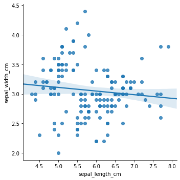
Imagine we want to predict sepal_width_cm based on sepal_length_cm: we may try fitting a simple linear regression model. The result is somewhat unsatisfying:

Fit a joint model

sns.lmplot(x="sepal_length_cm", y="sepal_width_cm", data=df)

<seaborn.axisgrid.FacetGrid at 0x7f600c6d2ba8>

In sklearn, we can represent the model (in this case, a linear regression on selected features) as a pipeline:

simple_model = Pipeline([
    ("features", PandasValueSelector("sepal_length_cm")),
    ("lr", LinearRegression()),
])

simple_model.fit(df, df["sepal_width_cm"])

Pipeline(memory=None,
     steps=[('features', PandasValueSelector(columns='sepal_length_cm')), ('lr', LinearRegression(copy_X=True, fit_intercept=True, n_jobs=None,
         normalize=False))])

y_pred, y = simple_model.predict(df), df["sepal_width_cm"]
print(f"MSE = {mse(y, y_pred)}, MAE = {mae(y, y_pred)}")

MSE = 0.18610437589381357, MAE = 0.33122352979559877

lr = simple_model.named_steps['lr']
print(f"Intercept: {lr.intercept_:.2f}, slope: {lr.coef_[0]:.2f}")

Intercept: 3.42, slope: -0.06

Fit a model per category

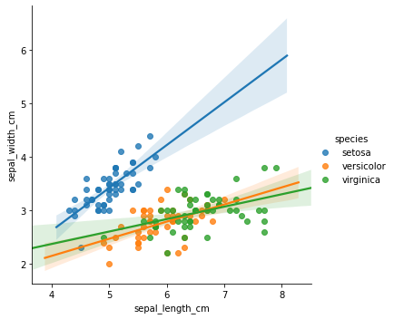
We can improve the regression model signiifcantly by adding the categorical feature species - we could try on-hot encoding, embeddings, etc. However, a common approach would be to fit a separate regression model per category:

sns.lmplot(x="sepal_length_cm", y="sepal_width_cm", hue="species", data=df)

<seaborn.axisgrid.FacetGrid at 0x7f600bee2860>

grouped_model = GroupedPipeline(
    groupby="species",
    pipeline=simple_model
)

grouped_model.fit(df, df["sepal_width_cm"])

# Specifying target by column name is also supported:
grouped_model.fit(df, "sepal_width_cm")

GroupedPipeline(errors='raise', groupby='species',
        pipeline=Pipeline(memory=None,
     steps=[('features', PandasValueSelector(columns='sepal_length_cm')), ('lr', LinearRegression(copy_X=True, fit_intercept=True, n_jobs=None,
         normalize=False))]))

y_pred, y = grouped_model.predict(df), df["sepal_width_cm"]
print(f"MSE = {mse(y, y_pred)}, MAE = {mae(y, y_pred)}")

MSE = 0.07119979049915942, MAE = 0.20655162210804365

for group, pipe in grouped_model.pipelines_.items():
    lr = pipe.named_steps['lr']
    print(f"{group}: intercept: {lr.intercept_:.2f}, slope: {lr.coef_[0]:.2f}")

setosa: intercept: -0.57, slope: 0.80
versicolor: intercept: 0.87, slope: 0.32
virginica: intercept: 1.45, slope: 0.23