This page was generated from docs/source/examples/SolarGenerationTimeSeries_Part1.ipynb.

Modelling Solar generation across Multiple Sites - Part 1

This example shows how timeserio helps building deep learning models for time series forecasting. Especially, we deal with the case of many related timeseries.

We demonstrate some core functionality and concepts, without striving for model accuracy or seeking out additional features like historic weather forecasts.

We will be using the dataset on solar (photo-voltaic, PV) generation potential across Europe, as collected by SETIS. The dataset presents solar generation, normalized to the solar capacity installed as of 2015.

Download the data

!mkdir -p ~/tmp/datasets; cd ~/tmp/datasets; wget https://setis.ec.europa.eu/sites/default/files/EMHIRES_DATA/Solar/EMHIRESPV_country_level.zip; unzip -o EMHIRESPV_country_level.zip; rm EMHIRESPV_country_level.zip

--2019-07-10 10:14:11--  https://setis.ec.europa.eu/sites/default/files/EMHIRES_DATA/Solar/EMHIRESPV_country_level.zip
Resolving setis.ec.europa.eu (setis.ec.europa.eu)... 139.191.207.52
Connecting to setis.ec.europa.eu (setis.ec.europa.eu)|139.191.207.52|:443... connected.
HTTP request sent, awaiting response... 200 OK
Length: 93401258 (89M) [application/zip]
Saving to: ‘EMHIRESPV_country_level.zip’

EMHIRESPV_country_l 100%[===================>]  89.07M  4.15MB/s    in 17s

2019-07-10 10:14:28 (5.16 MB/s) - ‘EMHIRESPV_country_level.zip’ saved [93401258/93401258]

Archive:  EMHIRESPV_country_level.zip
  inflating: EMHIRESPV_TSh_CF_Country_19862015.xlsx

Download data and save in a more performant format

import pandas as pd

%%time
df = pd.read_excel("~/tmp/datasets/EMHIRESPV_TSh_CF_Country_19862015.xlsx")

CPU times: user 1min 32s, sys: 268 ms, total: 1min 33s
Wall time: 1min 33s

df.head(3)

	Time_step	Date	Year	Month	Day	Hour	AL	AT	BA	BE	...	NO	PL	PT	RO	RS	SI	SK	SE	XK	UK
0	1	1986-01-01 00:00:00	1986	1	1	0	0.0	0.0	0.0	0.0	...	0.0	0.0	0.0	0.0	0.0	0.0	0.0	0.0	0.0	0.0
1	2	1986-01-01 01:00:00	1986	1	1	1	0.0	0.0	0.0	0.0	...	0.0	0.0	0.0	0.0	0.0	0.0	0.0	0.0	0.0	0.0
2	3	1986-01-01 02:00:00	1986	1	1	2	0.0	0.0	0.0	0.0	...	0.0	0.0	0.0	0.0	0.0	0.0	0.0	0.0	0.0	0.0

3 rows × 41 columns

Reshape data to tall format

We add a country column to identify each table row.

id_vars = ['Time_step', 'Date', 'Year', 'Month', 'Day', 'Hour']
country_vars = list(set(df.columns) - set(id_vars))
df_tall = pd.melt(df, id_vars=id_vars, value_vars=country_vars, var_name="country", value_name="generation")

Store to parquet

Apache Parquet is a much preferred data format for columnar numerical data - it is much faster to read (see below), is fully compatible with tools like pandas and Spark, and allows easy partitioning of large datasets.

%%time
df_tall.to_parquet("~/tmp/datasets/EMHIRESPV_TSh_CF_Country_19862015_tall.parquet")

CPU times: user 1.4 s, sys: 188 ms, total: 1.59 s
Wall time: 1.57 s

Store to partitioned parquet

%%time
df_tall.to_parquet("~/tmp/datasets/EMHIRESPV_TSh_CF_Country_19862015_partitioned/", partition_cols=["country"])

CPU times: user 3.07 s, sys: 806 ms, total: 3.88 s
Wall time: 3.46 s

!tree -h --filelimit=10 ~/tmp/datasets

/home/igor/tmp/datasets
├── [4.0K]  EMHIRESPV_TSh_CF_Country_19862015_partitioned [35 entries exceeds filelimit, not opening dir]
├── [123M]  EMHIRESPV_TSh_CF_Country_19862015_tall.parquet
└── [ 95M]  EMHIRESPV_TSh_CF_Country_19862015.xlsx

1 directory, 2 files

Load the data from parquet

import pandas as pd
import matplotlib.pyplot as plt
import seaborn as sns

%%time
df = pd.read_parquet("/tmp/datasets/EMHIRESPV_TSh_CF_Country_19862015_tall.parquet")

CPU times: user 888 ms, sys: 542 ms, total: 1.43 s
Wall time: 395 ms

print(' '.join(sorted(df['country'].unique())))

AL AT BA BE BG CH CY CZ DE DK EE EL ES FI FR HR HU IE IT LT LU LV ME MK NL NO PL PT RO RS SE SI SK UK XK

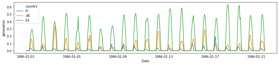
plot_countries = ['ES', 'UK', 'FI', ]

plt.figure(figsize=(15, 3))
sns.lineplot(
    data=df[(df['Time_step'] < 500) & (df['country'].isin(plot_countries))],
    x='Date', y='generation', hue='country',
)

<matplotlib.axes._subplots.AxesSubplot at 0x7f4df11a7c88>

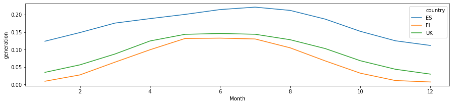
df_monthly = df.groupby(['Month', 'country']).mean().reset_index()

plt.figure(figsize=(15, 3))
sns.lineplot(
    data=df_monthly[df_monthly['country'].isin(plot_countries)],
    x='Month', y='generation', hue='country',
)

<matplotlib.axes._subplots.AxesSubplot at 0x7f1f9d9b6ba8>

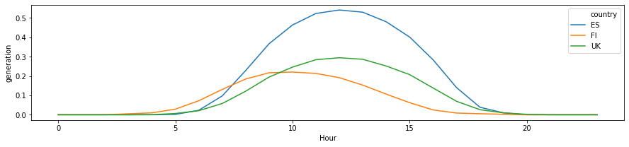
df_daily = df.groupby(['Hour', 'country']).mean().reset_index()

plt.figure(figsize=(15, 3))
sns.lineplot(
    data=df_daily[df_daily['country'].isin(plot_countries)],
    x='Hour', y='generation', hue='country',
)

<matplotlib.axes._subplots.AxesSubplot at 0x7f1f9d8dc128>

df_yearly = df.groupby(['Year', 'country']).mean().reset_index()

plt.figure(figsize=(15, 3))
sns.lineplot(
    data=df_yearly[df_yearly['country'].isin(plot_countries)],
    x='Year', y='generation', hue='country',
)

<matplotlib.axes._subplots.AxesSubplot at 0x7f1f9d855dd8>

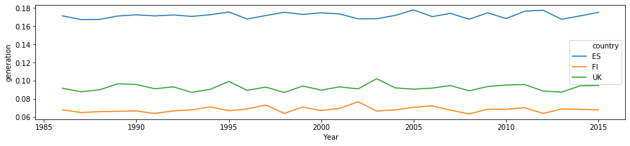
Preliminary observations

The timeseries for different countries exhibit a lot of similarity - they will have similar daily and seaonal shapes. At the same time, the curves have different scaling (due to latitudes and weather), and different time offsets (due to longitude). We can build models to incorporate these as external features, or learn the relevant features from the available data only!

Split into train-test sets

df_dev = df.iloc[:100]
df_train, df_test = df[df['Year'] < 1995], df[df['Year'] >= 1995]
len(df_train), len(df_test)

(2761080, 6442800)

Feature-based model with latent embeddings

For our first model, we use datetime and country as the only features.

To encode the datetime, we make use of periodic daily and yearly variables.

For each country, we learn an embedding, i.e. a latent representation, at training time.

Define feature preprocessing

Datetime encoding using periodic features

from timeserio.pipeline import Pipeline
from timeserio.preprocessing import (
    PandasValueSelector, PandasDateTimeFeaturizer, StatelessPeriodicEncoder
)

periodic_pipe = Pipeline([
    ('select', PandasValueSelector(['dayofyear', 'fractionalhour'])),
    ('encode', StatelessPeriodicEncoder(n_features=2, periodic_features='all', period=[365, 24])),
])

datetime_pipeline = Pipeline([
    ('featurize_dt', PandasDateTimeFeaturizer(
        column='Date', attributes=['dayofyear', 'fractionalhour'])),
    ('encode', periodic_pipe)
])

Country label encoding

We convert countries to integer labels

from sklearn.preprocessing import OrdinalEncoder

country_list = sorted(df['country'].unique())
country_encoder = OrdinalEncoder(categories=[country_list])
country_encoder.categories_ = [country_list] # we can also call .fit()

country_pipeline = Pipeline([
    ('select', PandasValueSelector("country")),
    ('encode', country_encoder)
])

Define the Neural Network Architecture

We define a regression network with two inputs: one for country feature, and one for datetime feature. It is easy to see how additional inputs can be added. The output is our prediction for PV generation in a given time and place.

from timeserio.keras.multinetwork import MultiNetworkBase

from keras.layers import Input, Dense, Embedding, Flatten, Concatenate
from keras.models import Model

class PVForecastingNetwork(MultiNetworkBase):
    def _model(
        self,
        location_dim=2, max_locations=100,  # embedding parameters
        num_features=4,  # number of real-valued features
        hidden_layers=2, hidden_units=8,  # any other parameters of the network
    ):
        loc_input = Input(shape=(1,), name='location')
        feature_input = Input(shape=(num_features,), name='features')
        loc_emb = Flatten()(Embedding(max_locations, location_dim, name='embed_location')(loc_input))
        output = Concatenate(name='concatenate')([loc_emb, feature_input])
        for idx in range(hidden_layers):
            output = Dense(hidden_units, activation='relu', name=f'dense_{idx}')(output)
        output = Dense(1, name='generation', activation='relu')(output)

        loc_model = Model(loc_input, loc_emb)
        forecasting_model = Model([loc_input, feature_input], output)
        forecasting_model.compile(optimizer='Adam', loss='mse', metrics=['mae'])

        return {'location': loc_model, 'forecast': forecasting_model}

multinetwork = PVForecastingNetwork()

Connect feature pipelines to the neural network

Now, we combine feature pre-processing pipelines with the neural network(s) for an encapsulated, reusable model object.

from timeserio.pipeline import MultiPipeline

First we define a helper MultiPipeline object to keep all pipelines in one place.

multipipeline = MultiPipeline({
    "country": country_pipeline,
    "datetime": datetime_pipeline,
    "target": PandasValueSelector("generation")
})

Now we can refer to the pipelines by names, and associate them with inputs and outputs of the keras models defined in PVForecastingNetwork:

from timeserio.multimodel import MultiModel

manifold = {
    # keras_model_name: (input_pipes, output_pipes)
    "location": ("country", None),
    "forecast": (["country", "datetime"], "target")
}

multimodel = MultiModel(
    multinetwork=multinetwork,
    multipipeline=multipipeline,
    manifold=manifold
)

Fit model from in-memory data

Having defined all details of our model in one place, fitting it is as simple as calling .fit() on a keras model:

multimodel.fit(df_train, model="forecast", batch_size=2 ** 16, epochs=50, verbose=1)

We can also use aby batch generator - the pre-processing pipelines will be applied to each batch, as long as the pipelines provide a .transform method:

batchgen = RowBatchGenerator(
    df=df_train, batch_size=2**15,
    columns=['Date', "country", "generation"],
    id_column="country",
    batch_aggregator=3
)
multimodel.fit_generator(batchgen, model="forecast", epochs=50, verbose=1, workers=8)

multimodel.fit(
    df_train, model="forecast", batch_size=2 ** 16, epochs=50, verbose=1,
    validation_data=df_test
)

Train on 2761080 samples, validate on 6442800 samples
Epoch 1/50
2761080/2761080 [==============================] - 4s 2us/step - loss: 0.0769 - mean_absolute_error: 0.1930 - val_loss: 0.0563 - val_mean_absolute_error: 0.1471
Epoch 2/50
2761080/2761080 [==============================] - 4s 1us/step - loss: 0.0528 - mean_absolute_error: 0.1327 - val_loss: 0.0513 - val_mean_absolute_error: 0.1238
Epoch 3/50
2761080/2761080 [==============================] - 4s 1us/step - loss: 0.0512 - mean_absolute_error: 0.1227 - val_loss: 0.0511 - val_mean_absolute_error: 0.1211
Epoch 4/50
2761080/2761080 [==============================] - 4s 1us/step - loss: 0.0512 - mean_absolute_error: 0.1213 - val_loss: 0.0511 - val_mean_absolute_error: 0.1205
Epoch 5/50
2761080/2761080 [==============================] - 4s 1us/step - loss: 0.0511 - mean_absolute_error: 0.1210 - val_loss: 0.0511 - val_mean_absolute_error: 0.1203
Epoch 6/50
2761080/2761080 [==============================] - 4s 1us/step - loss: 0.0511 - mean_absolute_error: 0.1208 - val_loss: 0.0510 - val_mean_absolute_error: 0.1201
Epoch 7/50
2761080/2761080 [==============================] - 4s 1us/step - loss: 0.0511 - mean_absolute_error: 0.1207 - val_loss: 0.0510 - val_mean_absolute_error: 0.1201
Epoch 8/50
2761080/2761080 [==============================] - 4s 1us/step - loss: 0.0510 - mean_absolute_error: 0.1206 - val_loss: 0.0509 - val_mean_absolute_error: 0.1200
Epoch 9/50
2761080/2761080 [==============================] - 4s 1us/step - loss: 0.0509 - mean_absolute_error: 0.1205 - val_loss: 0.0507 - val_mean_absolute_error: 0.1199
Epoch 10/50
2761080/2761080 [==============================] - 4s 1us/step - loss: 0.0461 - mean_absolute_error: 0.1149 - val_loss: 0.0256 - val_mean_absolute_error: 0.0947
Epoch 11/50
2761080/2761080 [==============================] - 4s 1us/step - loss: 0.0183 - mean_absolute_error: 0.0821 - val_loss: 0.0143 - val_mean_absolute_error: 0.0699
Epoch 12/50
2761080/2761080 [==============================] - 4s 1us/step - loss: 0.0128 - mean_absolute_error: 0.0653 - val_loss: 0.0115 - val_mean_absolute_error: 0.0608
Epoch 13/50
2761080/2761080 [==============================] - 4s 1us/step - loss: 0.0103 - mean_absolute_error: 0.0567 - val_loss: 0.0098 - val_mean_absolute_error: 0.0545
Epoch 14/50
2761080/2761080 [==============================] - 4s 1us/step - loss: 0.0090 - mean_absolute_error: 0.0519 - val_loss: 0.0089 - val_mean_absolute_error: 0.0515
Epoch 15/50
2761080/2761080 [==============================] - 4s 1us/step - loss: 0.0083 - mean_absolute_error: 0.0492 - val_loss: 0.0084 - val_mean_absolute_error: 0.0497
Epoch 16/50
2761080/2761080 [==============================] - 4s 1us/step - loss: 0.0079 - mean_absolute_error: 0.0476 - val_loss: 0.0082 - val_mean_absolute_error: 0.0486
Epoch 17/50
2761080/2761080 [==============================] - 4s 1us/step - loss: 0.0077 - mean_absolute_error: 0.0464 - val_loss: 0.0080 - val_mean_absolute_error: 0.0477
Epoch 18/50
2761080/2761080 [==============================] - 4s 1us/step - loss: 0.0075 - mean_absolute_error: 0.0455 - val_loss: 0.0078 - val_mean_absolute_error: 0.0470
Epoch 19/50
2761080/2761080 [==============================] - 4s 1us/step - loss: 0.0073 - mean_absolute_error: 0.0447 - val_loss: 0.0077 - val_mean_absolute_error: 0.0464
Epoch 20/50
2761080/2761080 [==============================] - 4s 1us/step - loss: 0.0071 - mean_absolute_error: 0.0441 - val_loss: 0.0075 - val_mean_absolute_error: 0.0458
Epoch 21/50
2761080/2761080 [==============================] - 4s 1us/step - loss: 0.0070 - mean_absolute_error: 0.0436 - val_loss: 0.0074 - val_mean_absolute_error: 0.0453
Epoch 22/50
2761080/2761080 [==============================] - 4s 1us/step - loss: 0.0069 - mean_absolute_error: 0.0431 - val_loss: 0.0074 - val_mean_absolute_error: 0.0450
Epoch 23/50
2761080/2761080 [==============================] - 4s 1us/step - loss: 0.0069 - mean_absolute_error: 0.0428 - val_loss: 0.0073 - val_mean_absolute_error: 0.0447
Epoch 24/50
2761080/2761080 [==============================] - 4s 1us/step - loss: 0.0068 - mean_absolute_error: 0.0426 - val_loss: 0.0072 - val_mean_absolute_error: 0.0444
Epoch 25/50
2761080/2761080 [==============================] - 4s 1us/step - loss: 0.0067 - mean_absolute_error: 0.0423 - val_loss: 0.0072 - val_mean_absolute_error: 0.0442
Epoch 26/50
2761080/2761080 [==============================] - 4s 1us/step - loss: 0.0067 - mean_absolute_error: 0.0421 - val_loss: 0.0071 - val_mean_absolute_error: 0.0441
Epoch 27/50
2761080/2761080 [==============================] - 4s 1us/step - loss: 0.0067 - mean_absolute_error: 0.0419 - val_loss: 0.0071 - val_mean_absolute_error: 0.0439
Epoch 28/50
2761080/2761080 [==============================] - 4s 1us/step - loss: 0.0066 - mean_absolute_error: 0.0418 - val_loss: 0.0071 - val_mean_absolute_error: 0.0438
Epoch 29/50
2761080/2761080 [==============================] - 4s 1us/step - loss: 0.0066 - mean_absolute_error: 0.0417 - val_loss: 0.0071 - val_mean_absolute_error: 0.0437
Epoch 30/50
2761080/2761080 [==============================] - 4s 1us/step - loss: 0.0066 - mean_absolute_error: 0.0416 - val_loss: 0.0070 - val_mean_absolute_error: 0.0436
Epoch 31/50
2761080/2761080 [==============================] - 4s 1us/step - loss: 0.0066 - mean_absolute_error: 0.0415 - val_loss: 0.0070 - val_mean_absolute_error: 0.0436
Epoch 32/50
2761080/2761080 [==============================] - 4s 1us/step - loss: 0.0066 - mean_absolute_error: 0.0414 - val_loss: 0.0070 - val_mean_absolute_error: 0.0435
Epoch 33/50
2761080/2761080 [==============================] - 4s 1us/step - loss: 0.0065 - mean_absolute_error: 0.0414 - val_loss: 0.0070 - val_mean_absolute_error: 0.0434
Epoch 34/50
2761080/2761080 [==============================] - 4s 1us/step - loss: 0.0065 - mean_absolute_error: 0.0413 - val_loss: 0.0070 - val_mean_absolute_error: 0.0434
Epoch 35/50
2761080/2761080 [==============================] - 4s 1us/step - loss: 0.0065 - mean_absolute_error: 0.0412 - val_loss: 0.0070 - val_mean_absolute_error: 0.0433
Epoch 36/50
2761080/2761080 [==============================] - 4s 1us/step - loss: 0.0065 - mean_absolute_error: 0.0411 - val_loss: 0.0070 - val_mean_absolute_error: 0.0432
Epoch 37/50
2761080/2761080 [==============================] - 4s 1us/step - loss: 0.0065 - mean_absolute_error: 0.0410 - val_loss: 0.0069 - val_mean_absolute_error: 0.0432
Epoch 38/50
2761080/2761080 [==============================] - 4s 1us/step - loss: 0.0065 - mean_absolute_error: 0.0409 - val_loss: 0.0069 - val_mean_absolute_error: 0.0430
Epoch 39/50
2761080/2761080 [==============================] - 4s 1us/step - loss: 0.0064 - mean_absolute_error: 0.0408 - val_loss: 0.0069 - val_mean_absolute_error: 0.0430
Epoch 40/50
2761080/2761080 [==============================] - 4s 1us/step - loss: 0.0064 - mean_absolute_error: 0.0407 - val_loss: 0.0069 - val_mean_absolute_error: 0.0430
Epoch 41/50
2761080/2761080 [==============================] - 4s 1us/step - loss: 0.0064 - mean_absolute_error: 0.0407 - val_loss: 0.0069 - val_mean_absolute_error: 0.0429
Epoch 42/50
2761080/2761080 [==============================] - 4s 1us/step - loss: 0.0064 - mean_absolute_error: 0.0406 - val_loss: 0.0069 - val_mean_absolute_error: 0.0429
Epoch 43/50
2761080/2761080 [==============================] - 5s 2us/step - loss: 0.0064 - mean_absolute_error: 0.0405 - val_loss: 0.0069 - val_mean_absolute_error: 0.0428
Epoch 44/50
2761080/2761080 [==============================] - 4s 2us/step - loss: 0.0064 - mean_absolute_error: 0.0405 - val_loss: 0.0069 - val_mean_absolute_error: 0.0427
Epoch 45/50
2761080/2761080 [==============================] - 4s 1us/step - loss: 0.0064 - mean_absolute_error: 0.0404 - val_loss: 0.0068 - val_mean_absolute_error: 0.0427
Epoch 46/50
2761080/2761080 [==============================] - 4s 2us/step - loss: 0.0064 - mean_absolute_error: 0.0403 - val_loss: 0.0068 - val_mean_absolute_error: 0.0426
Epoch 47/50
2761080/2761080 [==============================] - 4s 2us/step - loss: 0.0064 - mean_absolute_error: 0.0403 - val_loss: 0.0068 - val_mean_absolute_error: 0.0426
Epoch 48/50
2761080/2761080 [==============================] - 4s 1us/step - loss: 0.0063 - mean_absolute_error: 0.0402 - val_loss: 0.0068 - val_mean_absolute_error: 0.0425
Epoch 49/50
2761080/2761080 [==============================] - 4s 1us/step - loss: 0.0063 - mean_absolute_error: 0.0402 - val_loss: 0.0068 - val_mean_absolute_error: 0.0425
Epoch 50/50
2761080/2761080 [==============================] - 4s 2us/step - loss: 0.0063 - mean_absolute_error: 0.0401 - val_loss: 0.0068 - val_mean_absolute_error: 0.0424

<timeserio.keras.callbacks.HistoryLogger at 0x7f4c23fa9da0>

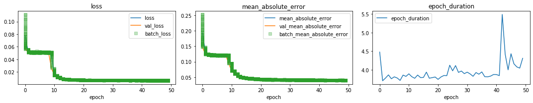
from kerashistoryplot.plot import plot_history
history = multimodel.history[-1]["history"]
plot_history(history, figsize=(15, 3), n_cols=3);

persist the model:

from timeserio.utils.pickle import loadf, dumpf
dumpf(multimodel, "/tmp/PV_model_1.pickle")

Look at predictions

%%time
df_test["prediction"] = multimodel.predict(df_test, model="forecast", batch_size=2**16, verbose=1)

6442800/6442800 [==============================] - 1s 0us/step
CPU times: user 4.88 s, sys: 970 ms, total: 5.85 s
Wall time: 4.53 s

/home/igor/.pyenv/versions/3.6.4/envs/data/lib/python3.6/site-packages/ipykernel_launcher.py:1: SettingWithCopyWarning:
A value is trying to be set on a copy of a slice from a DataFrame.
Try using .loc[row_indexer,col_indexer] = value instead

See the caveats in the documentation: http://pandas.pydata.org/pandas-docs/stable/indexing.html#indexing-view-versus-copy
  """Entry point for launching an IPython kernel.

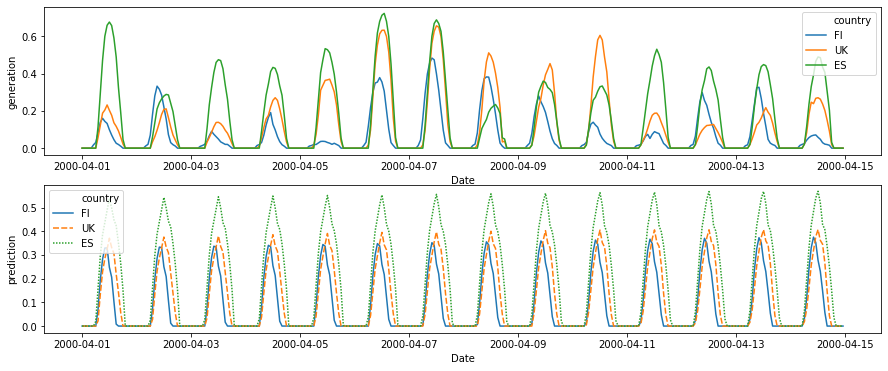
fig, axes = plt.subplots(nrows=2, figsize=(15, 6))
df_plot = df_test[(df_test['Year'] == 2000) & (df_test['Month'] == 4) & (df_test['Day'] < 15) & (df_test['country'].isin(plot_countries))]

sns.lineplot(
    data=df_plot,
    x='Date', y='generation', hue='country',
    ax=axes[0]
)

sns.lineplot(
    data=df_plot,
    x='Date', y='prediction', hue='country',
    style='country',
    dashes=True,
    ax=axes[1]
)

<matplotlib.axes._subplots.AxesSubplot at 0x7f4c943eaf98>

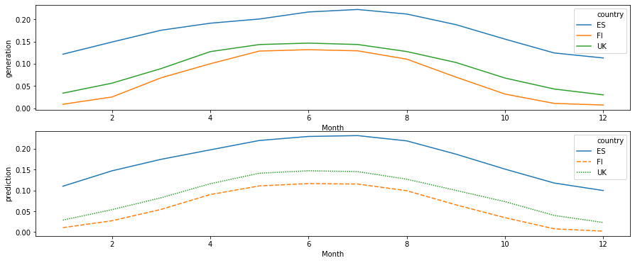
df_monthly = df_test.groupby(['Month', 'country']).mean().reset_index()

fig, axes = plt.subplots(nrows=2, figsize=(15, 6))
sns.lineplot(
    data=df_monthly[df_monthly['country'].isin(plot_countries)],
    x='Month', y='generation', hue='country',
    ax=axes[0]
)
sns.lineplot(
    data=df_monthly[df_monthly['country'].isin(plot_countries)],
    x='Month', y='prediction', hue='country',
    style='country',
    dashes=True,
    ax=axes[1]
)

<matplotlib.axes._subplots.AxesSubplot at 0x7f4c94071908>

df_daily = df_test.groupby(['Hour', 'country']).mean().reset_index()

fig, axes = plt.subplots(nrows=2, figsize=(15, 6))
sns.lineplot(
    data=df_daily[df_daily['country'].isin(plot_countries)],
    x='Hour', y='generation', hue='country',
    ax=axes[0]
)
sns.lineplot(
    data=df_daily[df_daily['country'].isin(plot_countries)],
    x='Hour', y='prediction', hue='country',
    style='country',
    dashes=True,
    ax=axes[1]
)

<matplotlib.axes._subplots.AxesSubplot at 0x7f4c8e4fd128>

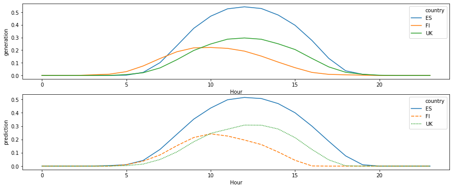
While our predictions do not capture short-range weather changes, they are excellent at seasonal level. Remember that all features such as location-specific scaling and time difference has been learned from the data!

Inspect the country embedding variables

We can inspect what the model learned about individual countries by inspecting the individual embeddings using multimodel:

multimodel.model_names

['location', 'forecast']

country_df = df_test.groupby("country")['generation', 'prediction'].mean().reset_index()
country_df.head(3)

	country	generation	prediction
0	AL	0.167597	0.173074
1	AT	0.125796	0.126038
2	BA	0.134952	0.136902

embeddings = multimodel.predict(country_df, model="location")

fig, ax = plt.subplots(figsize=(10, 10))
embeddings2 = pd.np.dot(embeddings, [[0, 1], [-1, 0]])
sns.scatterplot(x=embeddings2[:, 0], y=embeddings2[:, 1], size="generation", hue="generation", data=country_df, ax=ax)
for country, embedding in zip(country_list, embeddings2):
    ax.annotate(country, xy=embedding, xytext=embedding + 0.02)

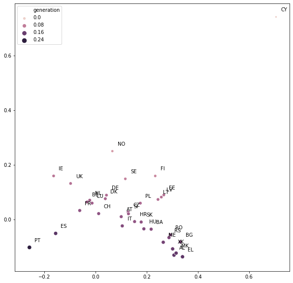
Note how similar the embeddings for BE, NL, LU and LT, LV, EE are! In fact, after a small (and arbitrary) rotation, we recover the map of Europe!

In this example, we have implemented a timeseries forecasting model using purely exogenous features, and made use of latent variables to capture the behaviour of multiple.